Excel: Use Sequence to Loop Through Characters

Recently, I was answering a question about how to write a formula that would reverse the letters in a cell. Excel doesn’t offer a simple =REVERSE(A2) formula. My traditional method for solving this is a custom VBA function that loops from the LEN(A2) to 1 and builds the answer backwards. Over the past five years, several newer methods have emerged:

• Power Query offers a Text.Reverse function.
• Excel VBA offers a StrReverse function.
• The new LAMBDA function could be used to call itself recursively.

Using Power Query means that the solution won’t work on a Mac. Using VBA means that the solution won’t work in Excel Online. The LAMBDA functions are still in beta and, frankly, can be difficult to understand.

THE SEQUENCE FUNCTION

The often-overlooked SEQUENCE function provides a solution that will work across all platforms. Given that Dynamic Arrays are out of beta, anyone with an up-to-date Microsoft 365 subscription will be able to use the formula.

The syntax for SEQUENCE is =SEQUENCE(rows,[columns],[start],[step]).

Here are some examples:

• =SEQUENCE(10) will generate a column of the numbers 1 through 10.
• =SEQUENCE(5,2) will generate the numbers 1 through 10 in a 2-column by 5-row range.
• =SEQUENCE(10,,,2) will generate the odd numbers 1 through 19.
• =SEQUENCE(10,5,500,-5) will generate 10 rows and 5 columns starting from 500 and counting backwards by 5.

HEAVY LIFTING WITH SEQUENCE

If you go back decades in Excel, there’s a little-known concept called “lifting.” If a function is expecting a single argument and you manage to pass it an array of arguments, the function will calculate once for each item in the array. You rarely saw this happen in legacy Excel because either implicit intersection or array truncation would prevent you from seeing all the answers.

But today, implicit intersection is turned off by default in Excel, and the ability for a single formula to spill into adjacent cells eliminates array truncation.

People have begun to realize that you can use a SEQUENCE formula as the argument to most Excel functions that expect a single value and cause the function to calculate multiple times.

In Figure 1, cell A2 contains the 26 letters of the alphabet arranged backwards. Normally, using =MID(A2,5,1) would extract the fifth character from the cell (in this case, V). But you don’t want just the fifth letter. You want all of the letters, and you want them in reverse sequence.

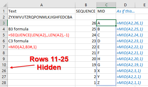
The formula =SEQUENCE(26,,26,-1) would generate 26 cells in a column, with the numbers starting at 26 and counting down to 1. To make this formula more flexible, you could use LEN(A2) instead of 26. That way, as the phrase entered in A2 changes, the formula will adapt to more or fewer letters.

In Figure 1, you can see two temporary formulas in cells B3 and C3. The formula in B3 generates the numbers 26 to 1 in a column.

The actual lifting happens in C3. This formula asks for the MID(A2,B3#,1). For the second argument, you aren’t passing it a single value. The B3# notation says that you want the entire array generated by the formula in B3. Normally, MID is expecting a single value as the second argument. When you cleverly force 26 values there, the MID function calculates 26 times and generates 26 results. It would be as if you actually typed the 26 formulas over in column D, but it all happens automatically thanks to lifting.

You can combine the formula in cells B3 and C3 into a single formula: =MID(A2,SEQUENCE(LEN(A2),,LEN(A2),-1)). This one formula would generate the 26 letters in reverse order.

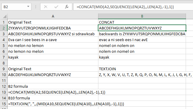
The final bit of magic is to send the 26 intermediate answers into a wrapper function such as TEXTJOIN or CONCAT. You could use TEXTJOIN if you wanted a comma and a space between each letter. To simply join everything together, it’s easier to use CONCAT.

Thus, =CONCAT(MID(A2,SEQUENCE(LEN(A2),,LEN(A2),-1))) becomes the function to reverse the text. Figure 2 shows the formula working with several phrases.

Reversing text is a niche need in Excel. But the concept of causing any function to calculate repeatedly by replacing an argument with the SEQUENCE function can be useful in many scenarios in Excel. Imagine calculating interest payments using IPMT for all 12 months of the year by passing a SEQUENCE(12) as the period argument to IPMT. You would likely wrap the IPMT function in a SUM function in order to book the interest expense for the year. The uses for this apporach of using SEQUENCE to lift a function are endless.

SF SAYS

SEQUENCE is a convenient way to generate an array of any size to force Excel to return a similar-sized array of answers.