But what if you wanted to calculate the maximum minus the minimum for each product? With a typical pivot table, the calculation fails because Excel calculates MAX minus MIN on a row-by-row basis in the original data.
Here’s a very simple example of why this calculation fails. Let’s say you’re tracking sales of fruit. Your data has four columns showing product, quantity, price for each item, and the total sale. Currently, there are exactly two rows of data. In row 2, you sold 1 case of bananas for $20. In row 3, you sold 100 cases of bananas for $8 each. The MIN price is $8, the MAX price is $20, and the delta between MIN and MAX is $12. But a regular pivot table would calculate the delta for row 2 as $20 ‒ $20, or $0. It would then calculate the delta for row 3 as $8 ‒ $8. The total delta for the data set will be $0.
There’s a powerful but obscure alternate formula language for pivot tables called DAX. To use it, you must choose to base your pivot table on the Data Model while creating the pivot table. The advantage of DAX is that the calculation happens once for each row in the final pivot table. Using DAX, Excel will calculate the MIN for all banana rows as $8, then calculate the MAX for all banana rows as $20. After those calculations are complete, DAX will calculate $20 ‒ $8 and come up with the accurate delta of $12. (Currently, the Data Model is only available in Excel for Windows. It isn’t yet working in Excel Online, Excel for Android, Excel for iOS, or Excel for Mac.)
USING THE DATA MODEL
To use the Data Model for your pivot table, select one cell in your detailed data. From the Insert tab, choose Pivot Table, From Table or Range to open the Pivot Table dialog box. At the bottom of that dialog is a checkbox for “Add this data to the Data Model.” Choose this box and then click OK.
Build the pivot table as normal. Drag Product to the Rows area. Drag the Each price to the Values area twice. Double-click the heading cell for the first Sum of Each to open the Value Field Settings dialog. In that dialog, change the “Summarize Value Field By” from Sum to Min. Click OK.
Double-click the heading cell for the Sum of Each2 column. Change the calculation to Max. Change the custom name from “Max of Each2” to “Max of Each.”
ADDING A DAX CALCULATION
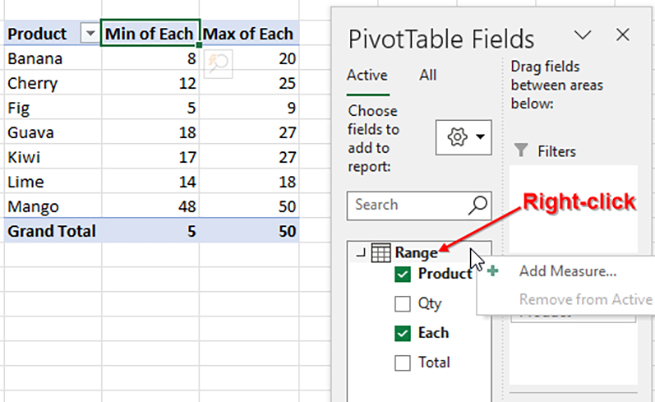
Figure 1 shows the PivotTable Fields pane when the pivot table is based on the Data Model. The original data set has four fields—Product, Qty, Each, and Total—that appear indented in the Fields pane under the word “Range.” The key to creating a DAX calculated field is to right-click the word Range and then choose Add Measure.
Note that the SQL Server developers who created the DAX language use the term “Measure” instead of “Calculated Field.” For a few early years, the DAX formulas were called “Calculated Field” in Excel, but this was too confusing because legacy pivot tables also have a “Calculated Field” feature. To differentiate the better DAX formulas from the legacy formulas, Microsoft chose to use the term “Measure,” even though it isn’t meaningful for most Excel users.
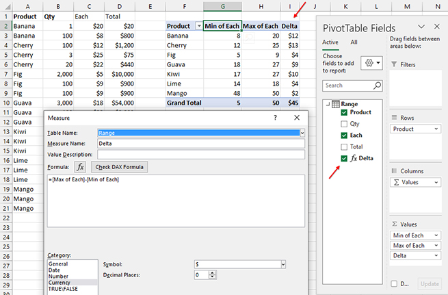
The Measure dialog box starts with a Table Name of “Range.” You get to fill in the Measure name. In Figure 2, I’ve used “Delta.” The Formula box begins with an equal sign. Click after the equal sign and type a left square bracket ([), and a selection box appears. You’ll see all of the fields in the original data set plus one calculated field for each item in the Values area. Double-click [Max of Each] to insert it into the formula. Click after =[Max of Each]. Type a minus sign and type another left square bracket to open the selection box. This time, choose [Min of Each] and press Tab to insert it into the formula.
You also have the option to specify the number format as Currency with 0 decimal places. The dialog also contains a button labeled Check DAX Formula. You can click that to make sure the formula is valid.
Once you’re ready, click OK to add the new calculation to the PivotTable Fields list. It will appear with a script “fx” logo and the field name of Delta.
You will have to select the checkbox next to fx Delta in order to add the calculation to the pivot table.
For the pivot table in Figure 2, the Delta formula is only used eight times. Being able to perform a calculation on the summary numbers shown in the pivot table adds a lot of functionality that goes beyond regular pivot tables.
There are many other scenarios where you need to wait to perform a calculation on the summary numbers elsewhere in the pivot table. In many of these situations, adding the data to the Data Model and then using a DAX measure will allow you to perform calculations inside of the pivot table instead of trying to perform these calculations outside of the pivot table.

February 2023


