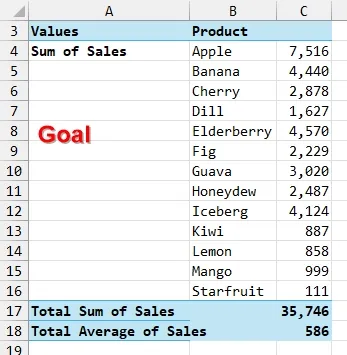
A manager recently asked if a pivot table could show sales detail by product and average sales, not for each product, but just one average for the entire data set. While the easy way is to hide some rows, you can also use an obscure language to solve this problem.
The language is called MDX, or Multidimensional Expressions. There is one entry point in the pivot table interface to write or edit MDX.
Figure 1
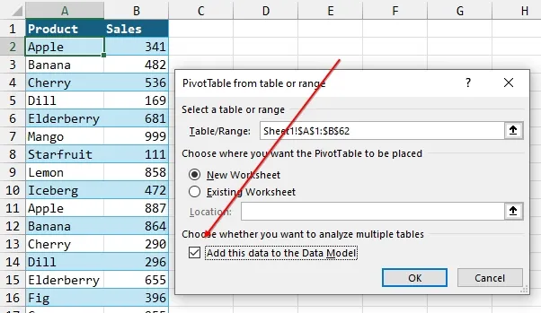
MDX is only available in pivot tables based on an external data set or on the data model in Excel. The simplest way to create a pivot table that uses the Data Model is to select the checkbox for “Add this data to the Data Model” when you create the pivot table.
Figure 2
With this particular data set, add Product to the Rows area and Sales to the Values area. That creates a pivot table that looks like this one:

Figure 3
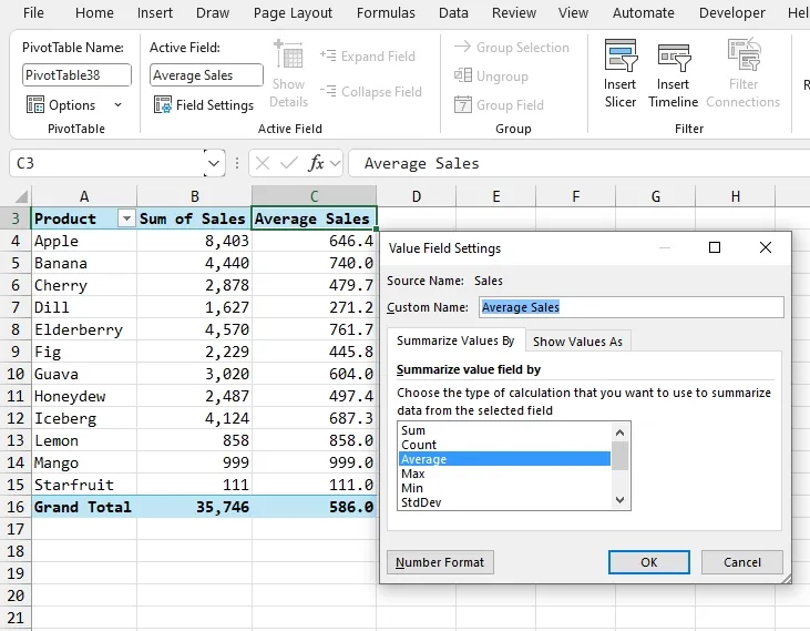
Your next goal is to add Average Sales to the pivot table. Drag the Sales field from the field list and drop it as a second Sales field in the Values area of the pivot table. This field will initially be called Sum of Sales2. Double-click the heading for Sum of Sales2. Change the calculation from Sum to Average. Change the field name from Sum of Sales2 to Average Sales, as shown in Figure 4.
Figure 4
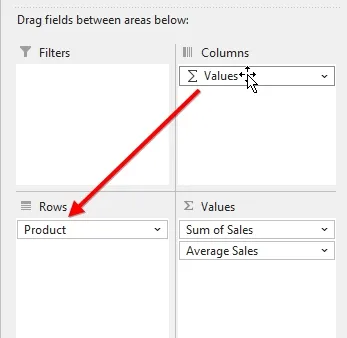
After you have multiple fields in the Values area of a pivot table, a virtual field called Values appears in the Columns area of the pivot table. Drag this field from Columns and drop it above the first Rows field, as shown in Figure 5.
Figure 5
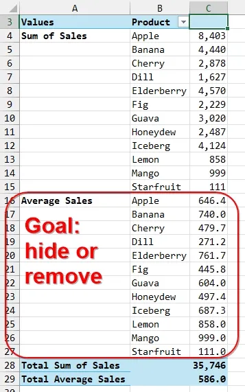
After moving Values to be the first Rows field, you should see a pivot table like the one shown in Figure 6. Your goal is to keep the Product details in rows 4 to 15, hide the Average details in rows 16 to 27, and then keep the totals from rows 28 and 29.
Figure 6
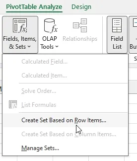
The obscure way to hide rows in a pivot table is to “Create a Set Based on Row Items.” This feature only works on pivot tables that use the Data Model. Select a cell in the Rows area of the pivot table. Go to the PivotTable Analyze tab in the ribbon. Open the Fields, Items, & Sets drop-down menu to select “Create Set Based on Row Items,” as shown in Figure 7.
Figure 7
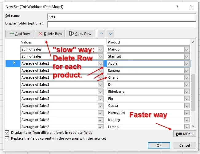
Figure 8 shows the New Set dialog box. Each row in the pivot table is represented by drop-downs showing the field names. Figure 8 has scrolled past most of the Sales details and is now showing the first Averages for individual products.
The “normal” way of using this dialog is to select the row for Average of Sales2 for Apple, then click the Delete Row button at the top. It is tedious, but you select each individual average product row and, for each, select Delete Row.
However, in this article, I am showing you how to skip those steps and write MDX to describe which rows should be included in the pivot table.
In the lower right corner, click Edit MDX….
Figure 8
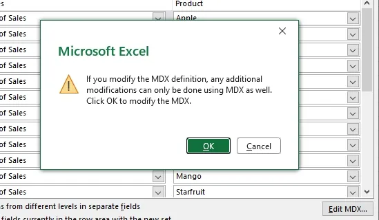
Microsoft warns you that once you modify the MDX, any further changes to this set will have to be made through MDX and not using the interface shown in Figure 8. Select OK to acknowledge this message.
Figure 9
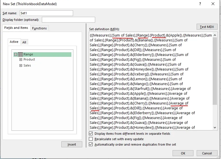
After editing the MDX, you can see the MDX for your current pivot table. You are going to delete all of this MDX code, but before you do, you can learn some valuable things from the code. I've added the red underlines to Figure 10 to show the important bits of the code.
- The name of the source table is called
[Range]. - The name of the first field in the Values area is called
[Sum of Sales]. - The name of the second field in the values area is called
[Average of Sales]. - The name of the row field is
[Product].
The current MDX lists all of the current products, by repeating code that look like this:
[Measures].[Sum of Sales].[Range].[Product].&[Apple]
This is not a safe solution, because a future pivot table might have new products.
Figure 10
Select and delete the MDX code shown in Figure 10.
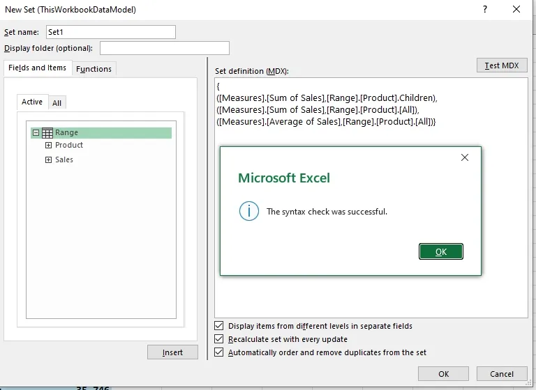
Replace it with this MDX code:
{([Measures].[Sum of Sales],[Range].[Product].Children),

([Measures].[Sum of Sales],[Range].[Product].[All]),

([Measures].[Average of Sales],[Range].[Product].[All])}
In this code the line ending with .Children will show the Sum of Sales for each Product. The second line shows the total row for Sum of Sales. The third line shows the total row for Average of Sales.
In the top right corner, click the Test MDX button. Excel will confirm if your MDX is valid, as shown in Figure 11.
Click OK to close the Syntax check. Click OK to close the New Set dialog.
Figure 11
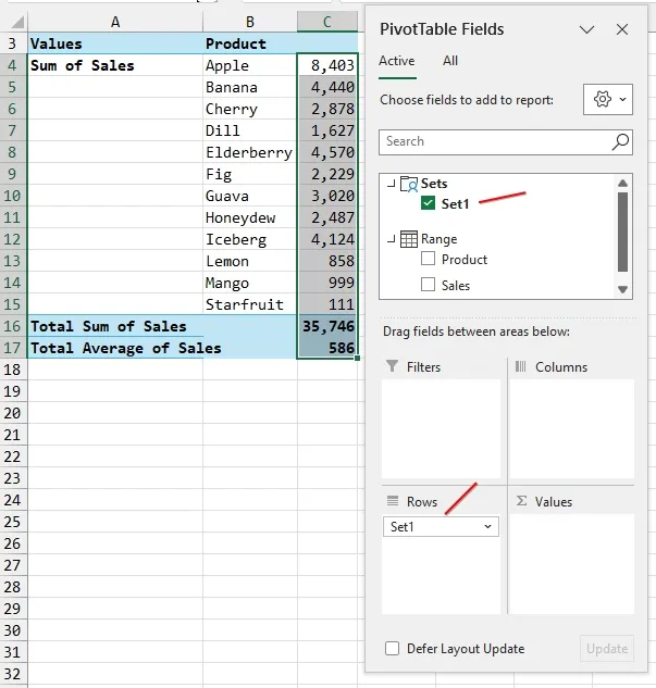
Something new appears in the PivotTable Fields pane. A new category called Sets is shown at the top with a set called Set1. This item is selected instead of the previous settings of Product and Sales.
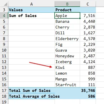
The pivot table shown in Figure 12 achieves the goal of showing each Product for Sum of Sales, followed by Grand Total Sales and an average across all products.
Figure 12
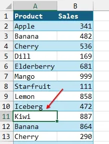
The advantage of the new MDX code is the flexibility to deal with new products. To test this, go back to the source data. Change A11 from Apple to Kiwi. This introduces a new product that is not in the original data.
Figure 13
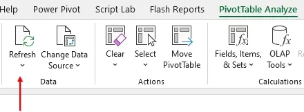
On the PivotTable Analyze tab, select Refresh, as shown in Figure 14. The pivot table should update, showing the new product (Kiwi).
Figure 14
Figure 15
Why have most people never heard of MDX or of Sets in pivot tables? The main reason is that Sets are greyed out when your pivot table is not based on the Data Model. Since most pivot tables use a regular pivot cache, you likely have not had the opportunity to use Sets in the past. By choosing to add the data to the Data Model, you’ve unlocked amazing new functionality.


