Excel: Text to Columns with TEXTSPLIT

But a deeper dive reveals that the arguments available in TEXTSPLIT also offer additional functionality.

USING TEXTSPLIT

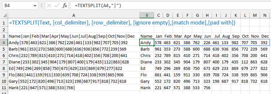
The function’s syntax is =TEXTSPLIT(text,col_delimiter,[row_delimiter],[ignore_empty],[match_mode],[pad_with]). In its simplest use, you pass the function some text and specify the delimiter. Figure 1 has several values separated by a pipe character (|). Using =TEXTSPLIT(A3,"|") breaks the 13 values from cell A3 into a horizontal row of 13 values.

Instead of breaking text into new columns, you can specify a row delimiter and break text into new rows. If you had a paragraph of sentences in A3, for example, =TEXTSPLIT(A3,, ".") would generate a vertical array of the sentences.

A paragraph might contain sentences that end with a variety of punctuation. If you want to handle text that could contain periods, question marks, and exclamation marks, enclose the three row delimiters in curly braces: =TEXTSPLIT(A3,,{".", "?","!"}).

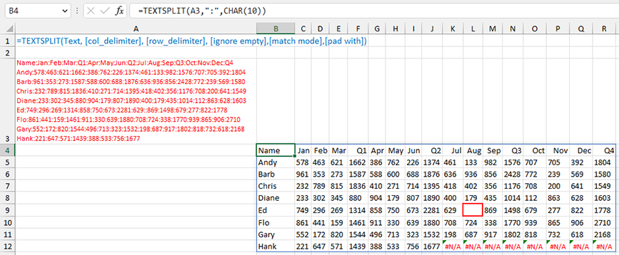
It’s also possible to specify both a column and row delimiter. In Figure 2, the entire data set is enclosed in cell A3. Each month is separated by a colon, and each row ends with a linefeed character (to create a line break within the cell). Someone could have typed this data in Excel by using Alt+Enter after each row to insert the linefeed, or they could have typed it in Word and included a carriage return at the end of each row. Linefeeds appear in Excel as CHAR(10), and carriage returns are CHAR(13). You could experiment with:

=TEXTSPLIT(A3,":",CHAR(10))

=TEXTSPLIT(A3,":",CHAR(13))

=TEXTSPLIT(A3,":",{CHAR(10),
CHAR(13)})

There are a couple of oddities in Figure 2 that can be controlled with the optional TEXTSPLIT arguments.

Notice that Hank only has data through Q2. When Excel sees that the longest row contains 17 values, it defaults to making all rows have 17 values. Excel can’t make up the missing Hank values, so it fills those cells with #N/A. This will cause problems later. Control this with the optional Pad With argument. Specify a 0 to replace missing values with zero. Specify “” to fill empty cells with blanks.

Also note that Ed’s August value is missing. In the original data, Ed shows 629::869. By default, Excel will assume the consecutive delimiters mean there should be a value there. That’s correct in this case, but there are situations where consecutive delimiters shouldn’t create a new value, like if you were separating each word into a new cell and accidentally added two spaces between a pair of words. Setting the optional Ignore Empty argument to True avoids an empty cell being returned.

Finally, there’s the optional Match Mode argument. If you have a delimiter that’s alphabetic, such as A, a, Z, or z, you can specify if the delimiter is case-sensitive: Use a 0 for the delimiter to be case-sensitive and 1 for it to be case-insensitive.

HOW TO SKIP CERTAIN COLUMNS

Step 3 of the Text to Columns wizard lets you select “Do Not Import” to skip certain columns. What if you wanted only the Names and Quarter totals from Figure 2? Microsoft introduced these new functions along with TEXTSPLIT:

• TAKE keeps only the first or last row(s) or column(s) from an array.
• DROP removes the first or last row(s) or column(s) from an array.
• CHOOSEROWS keeps a specific list of rows.
• CHOOSECOLS keeps a specific list of columns.

Which one to use depends on the shape of the data. Since the current example requires you to keep the columns 1, 5, 9, 13, and 17, which aren’t at the beginning or end, you can’t use TAKE or DROP. One option is to specify the column number at the end of CHOOSECOLS:

=CHOOSECOLS(TEXTSPLIT(A3,":",CHAR(10),,,0),1,5,9,13,17).

Since there’s a pattern in the numbers (1, 5, 9, 13, 17), you can use SEQUENCE to start at 1 and increment by 4 columns: =SEQUENCE(5,,1,4). Instead of typing the column numbers, you could use:

=CHOOSECOLS(TEXTSPLIT(A3,":",CHAR(10),,,0),SEQUENCE(5,,1,4)).