Hierarchies are one of the least discoverable features of a pivot table. By setting up a hierarchy, you can drill down into the pivot table without using filters or slicers.
Consider the data shown in Figure 1. There’s an obvious geographic hierarchy with fields for Continent, Country, Region, Territory, and City.
The hierarchy feature requires your data to be stored in the workbook’s Data Model. You could do this with Power Query, but the easiest way is to convert the data from Figure 1 into a table. With one cell in the data selected, press Ctrl+T. In the Create Table dialog, make sure that the box for My Data Has Headers is selected.
Excel will convert your data to a table and give it a name such as Table1. You can optionally rename the table using the Table Design tab in the ribbon; however, it’s fine to leave it as Table1.
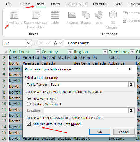
On the Insert tab, choose PivotTable. In the PivotTable dialog box, select the checkbox for “Add this data to the Data Model (see Figure 2).
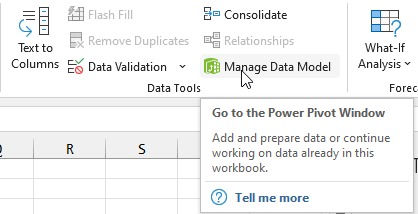
On the Data tab, toward the right in the Data Tools group, click Manage Data Model (see Figure 3). In older versions of Excel, this icon was only found on the Power Pivot tab in the ribbon.
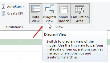
When you click Manage Data Model, you’re taken to the Power Pivot view of the grid. In the top right is an icon to display the Diagram View (see Figure 4). Click that icon to display a data diagram.
The Diagram View will display the fields in Table1. Initially, the box is large enough to show five fields. Drag the bottom of the box down to show the remaining fields with enough extra room for one more row.
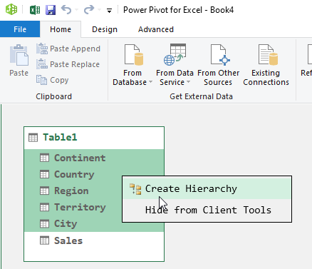
Click on Continent as it’s the first field for the hierarchy. Then shift-click on City as it is the final field of the hierarchy. All five fields will have green shading applied. Right-click anywhere in the green shading and select Create Hierarchy (see Figure 5). Note that if the fields for your hierarchy aren’t adjacent to each other, you could select the first field and then Ctrl+click the remaining fields.
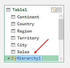
A new row appears at the bottom of the table as shown in Figure 6. The name is initially Hierarchy1, but the name is selected in edit mode so you can easily type a new name.
Type a name for the hierarchy, such as Geography, and press Enter.
As soon as you add the hierarchy in the Data Model, the Excel worksheet displays a warning that the Data Model has changed. It tells you to select the worksheet in order to see the updates in the PivotTable Fields pane. Since the Power Pivot window is often not full-screen, you might notice this warning bar in Excel. It’s normal and nothing to be concerned about.
In the Power Pivot window, choose File, Close to close the Power Pivot window and return to the worksheet in Excel.
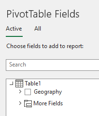
The PivotTable Fields pane now shows the Geography hierarchy and More Fields (see Figure 7). Your Sales field is hidden under More Fields. I understand and agree with Microsoft hiding Continent, Country, Region, Territory, and City under More Fields, but it seems buggy that the Sales field is hidden under More Fields.
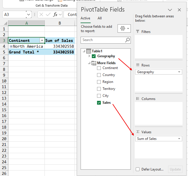
Click the arrow to the left of More Fields to expand it. Choose Sales to move it to the Values area. Choose Geography to move it to the Rows Area. The resulting pivot table shows just North America and $334 million (see Figure 8).
Right-click the numeric cell in the pivot table. Choose Number Format. Apply your desired currency or number format.
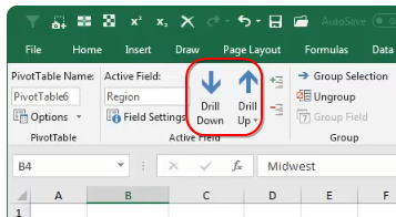
If you have an older version of Excel, you’ll see Drill Down and Drill Up buttons in the PivotTable Analyze tab of the ribbon (see Figure 9). These icons were there in Excel 2016 and Excel 2019 but have been hidden in Microsoft 365.
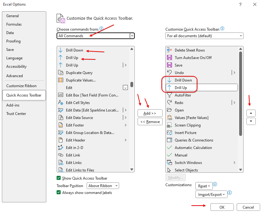
To bring back the Drill Down and Drill Up functionality, follow these steps to add the icons to the Quick Access Toolbar.
Right-click the Quick Access Toolbar and choose Customize the Quick Access Toolbar. This opens the Excel Options dialog and chooses the Quick Access Toolbar category.
Find the top-left drop-down menu that currently shows Popular Items. Open that drop-down and choose All Commands.
Scroll through the left list box until you find Drill Down and Drill Up. One at a time, click the icon on the left and then click the Add>> button in the middle of the screen. Optionally, use the up arrow button on the right side of the screen to move the icons to an earlier position on the Quick Access Toolbar. Finally, click OK (see Figure 10).
Drilling Through the Hierarchy
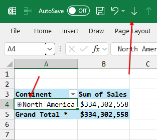
Click on North America in cell A4. The Drill Down icon is now enabled (see Figure 11).
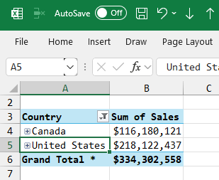
Drill down on North America. Excel replaces North America with two rows, one for Canada and one for the United States (see Figure 12).
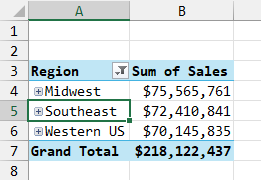
Click on United States and drill down again. The countries are removed, and you will see three regions for the U.S. (see Figure 13).
Click on the Southeast region and drill down two more times. You will see Figure 14 and then Figure 15.
Now that you’ve reached the final level of the hierarchy, you will use the Drill Up icon to return to previous levels.
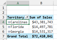
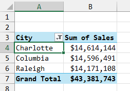
What is the advantage of the hierarchy? After all, regular pivot tables offer the Expand and Collapse buttons. But if I want to show only the cities in the Carolinas, you’d have to have used a slicer or Report Filter to remove the other territories.
Why Did Microsoft Hide the Drill Down and Drill Up Buttons?
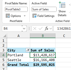
The hierarchy feature was rarely used. This isn’t surprising, particularly since the entry point for creating a hierarchy can only be found while managing the Data Model. In early 2024, Microsoft removed the Drill Down and Drill Up icons and replaced them with a new icon called Show Details (see Figure 16). This icon is the same as double-clicking any number in the pivot table. A new worksheet is inserted with the rows that make up the number.
One nice enhancement: The Show Details report now includes a title that explains which items are represented (see Figure 17).
With certain data sets, the Drill Down and Drill Up buttons provide an innovative way to analyze your data. It’s worth the extra steps to build the hierarchy in the Data Model to enable this feature.

February 2024


