

Kelly asks if there’s a way to protect a worksheet so other people can’t unhide certain columns. The process isn’t intuitive, and there’s a chance that a clever person could use formulas to learn the data in the hidden columns.
Every cell in the worksheet has a property called “Locked.” This setting has no effect until you protect the worksheet. It seems counterintuitive, but every cell on every worksheet begins with the Locked property set to On. A good first step is to select all cells in the worksheet and clear the Locked property to unlock all cells.
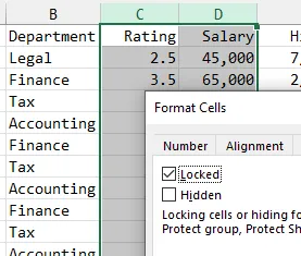
You can select all cells by clicking the triangle above and to the left of cell A1. With all cells selected, press Ctrl+1 to display the Format Cells dialog box. In the Format Cells dialog, choose the Protection tab. As shown in Figure 1, all the cells are currently locked. Uncheck the Locked status and click OK.
Figure 1

Next, you want to choose the columns that will eventually be hidden. In Figure 2, all of columns C and D are selected. You can do this by clicking on the column letter C and dragging over to the column letter D. With both columns selected, press Ctrl+1 to display the Format Cells dialog box. On the Protection tab, choose Locked to lock just these two columns. Click OK.
Figure 2
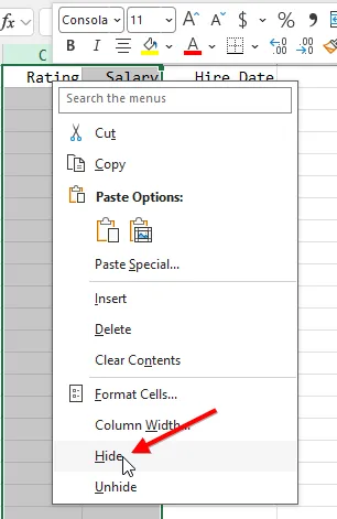
With both columns still selected, right-click any cell in the selection and choose Hide from the bottom of the menu that appears as shown in Figure 3.
Figure 3
At this point, anyone could easily unhide the columns. They could also use Ctrl+G or F5 to display the Go To dialog and select the hidden cells in columns C or D. Even with the columns hidden, you can see the current value in the formula bar and use the arrow keys to move up or down the hidden cells.
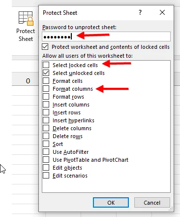
On the Review tab, choose Protect Sheet. Excel displays the Protect Sheet dialog as shown in Figure 4.
In the Protect Sheet dialog box, pay careful attention to several settings:
- The top choice for Select Locked Cells is enabled by default. You should uncheck this setting.
- The second choice for Select Unlocked Cells is enabled by default. Make sure this stays enabled.
- The fourth choice for Format Columns should not be enabled.
- Optionally, add a password in the box at the top. Adding a password is not foolproof. There are companies around the world that sell password-cracking utilities for many applications, including Excel. If you enter a password and click OK, you will have to re-enter the password one more time.
Figure 4
When you click OK to protect the sheet, people should be able to select any of the unlocked cells and edit them. However, they will not be able to hide or unhide any columns.
Not Perfect
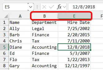
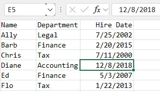
Take a look at the spreadsheet in Figure 5. Anyone could notice that the column headers jump from B to E. This might make them curious about what information is stored in C1, D1, and the other cells in those columns.
Figure 5
You might try to obscure that you have hidden columns by hiding the column letters. On the View tab, in the Show group, unselect the Headings as shown in Figure 6.
Figure 6
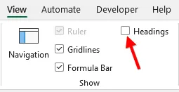
This hides the row numbers and column letters, making it less obvious that columns C and D are missing. However, the Name Box will still reveal that the third column is Column E and not Column C.
Figure 7
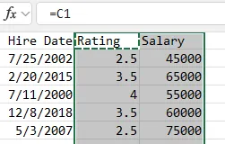
Once someone figures out that there might be secret information hidden in columns C & D, they could simply go to a blank section of the worksheet and enter a formula such as =C1. If they copied this formula to the bottom of the data and one column to the right, all of the hidden data would be revealed as shown in Figure 8.
Figure 8
One way to distribute the data without any chance of unhiding the data in the hidden columns is to use File, Export, Create PDF/XPS to create a PDF of the visible portions of the worksheet. The data in the hidden columns will not be available in the PDF.

